Heart Disease Predictor is a simple machine learning model that is designed to predict the likelihood of a patient having heart disease based on various input features.

The Heart Disease Predictor is typically trained on a large dataset of patient records, which includes features such as age, sex, blood pressure, cholesterol levels, and other relevant medical information. The model uses this data to learn patterns and relationships that can help predict the likelihood of heart disease in new patients.

Once the model is trained, it can take input data on a new patient and output a prediction of their likelihood of having heart disease. This information can be used by doctors and medical professionals to make more informed decisions about patient care and treatment.

Heart Disease Predictor can be a valuable tool in healthcare settings, helping to identify patients who are at high risk for heart disease and enabling early intervention and treatment. By using machine learning algorithms to analyze large amounts of medical data, Heart Disease Predictor can provide accurate and timely predictions that can improve patient outcomes and save lives.

Data Descrpition

Using this medical dataset,related to cardiovascular disease. Each row represents a patient, and each column represents a different attribute of the patient. Here's what each attribute means:

• age: the age of the patient in years
• sex: the biological sex of the patient (1 for male, 0 for female)
• cp: chest pain type (1 for typical angina, 2 for atypical angina, 3 for non-anginal pain, 4 for asymptomatic)
• trestbps: resting blood pressure (in mm Hg) upon admission to the hospital
• chol: serum cholesterol level (in mg/dl)
• fbs: fasting blood sugar > 120 mg/dl (1 for true, 0 for false)
• restecg: resting electrocardiographic results (0 for normal, 1 for having ST-T wave abnormality, 2 for showing probable or definite left ventricular hypertrophy by Estes' criteria)
• thalach: maximum heart rate achieved during exercise
• exang: exercise induced angina (1 for yes, 0 for no)
• oldpeak: ST depression induced by exercise relative to rest
• slope: the slope of the peak exercise ST segment (1 for upsloping, 2 for flat, 3 for downsloping)
• ca: number of major vessels (0-3) colored by fluoroscopy
• thal: a blood disorder called thalassemia (3 for normal, 6 for fixed defect, 7 for reversable defect)
• target: presence of heart disease (1 for yes, 0 for no)

Libraries

import numpy as np
import pandas as pd
import matplotlib.pyplot as plt
import seaborn as sns
%matplotlib inline 

# ML Models Scikit-Learn
from sklearn.linear_model import LogisticRegression
from sklearn.neighbors import KNeighborsClassifier
from sklearn.ensemble import RandomForestClassifier

# Model Evaluations
from sklearn.model_selection import train_test_split, cross_val_score
from sklearn.model_selection import RandomizedSearchCV, GridSearchCV
from sklearn.metrics import confusion_matrix, classification_report
from sklearn.metrics import precision_score, recall_score, f1_score
from sklearn.metrics import plot_roc_curve

Key Steps

1. Data Exploration

• Dataset contains 303 entries with 14 columns.
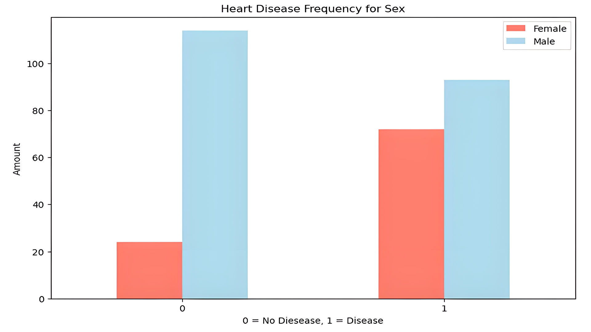
• The target variable indicates the presence (1) or absence (0) of heart disease.
• Sex distribution shows more males in the dataset:

2. Data Cleaning

• Checked for missing values: None found.
• Generated statistical summary using df.describe():
  • Average age: 54 years
  • Average cholesterol: 246 mg/dL

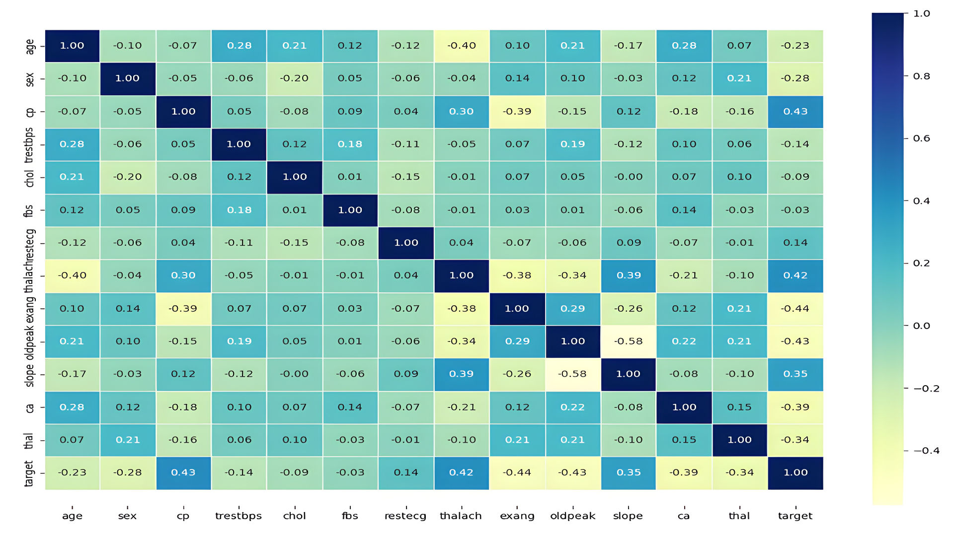
3. Data Visualization

• Correlation heatmap:

4. Machine Learning Models

Three models were implemented:

• Logistic Regression
• K-Nearest Neighbors (KNN)
• Random Forest Classifier

---

Logistic Regression

Logistic regression estimates the probability of an event occurring, such as voted or didn’t vote, based on a given data set of independent variables.

This type of statistical model (also known as logit model) is often used for classification and predictive analytics. Since the outcome is a probability, the dependent variable is bounded between 0 and 1. In logistic regression, a logit transformation is applied on the odds—that is, the probability of success divided by the probability of failure. This is also commonly known as the log odds, or the natural logarithm of odds, and this logistic function is represented by the following formulas:

Definition adapted from
What is logistic regression?

The logistic function (sigmoid function) is the core of logistic regression, defined as:

$${\sigma(z) = \frac{1}{1 + e^{-z}}}$$

Where $z$is a linear combination of input features, weights, and bias:

$${z = \mathbf{w}^T\mathbf{x} + b}$$

The logit transformation applies the natural logarithm to the odds of success ($p$):

$${\text{Logit}(p) = \log\left(\frac{p}{1-p}\right)}$$

Logistic regression minimizes the cross-entropy loss function to optimize the model's weights and bias.

Performance:

• Accuracy: 88.5%
• Strengths: Simple and interpretable; works well on linearly separable data.
• Limitations: Struggles with non-linear patterns without additional transformations or features.

---

K-Nearest Neighbors (KNN)

K-Nearest Neighbors is a simple, non-parametric algorithm used for classification and regression. It classifies a data point based on the majority class of its k nearest neighbors in the feature space.

Key Features:

1. Distance Metric: KNN uses a distance metric (e.g., Euclidean distance) to determine the proximity of points.
2. K Parameter: The hyperparameter $k$ determines the number of neighbors considered. A smaller $k$ may lead to overfitting, while a larger $k$ may smooth out the decision boundary.

Steps:

1. Calculate the distance from the test point to all training points.
2. Select the $k$ closest neighbors.
3. Assign the majority class among the neighbors to the test point.

Performance:

• Accuracy: 75.4% (optimized with $k=11`$).
• Strengths: Simple and effective; no need for explicit training.
• Limitations: Computationally expensive for large datasets; sensitive to feature scaling and irrelevant features.

Optimization:

Using Hyperparameter Tuning, $k$ was optimized by testing values from 1 to 20. The best test accuracy was achieved with $k=11$.

---

Random Forest Classifier

Random Forest is an ensemble learning method that combines multiple decision trees to improve classification accuracy and reduce overfitting. It uses bagging (Bootstrap Aggregating) and random feature selection to create a diverse set of trees.

Key Features:

1. Bagging: Each tree is trained on a bootstrap sample (random sample with replacement) of the data.
2. Random Feature Selection: At each split, the algorithm considers a random subset of features, ensuring diversity among the trees.
3. Voting: For classification, the forest outputs the majority vote of the individual trees.

Steps:

1. Train multiple decision trees on random subsets of data and features.
2. Aggregate predictions using majority voting (classification) or averaging (regression).

Performance:

• Accuracy: 83.6% (88.6% after hyperparameter tuning).
• Strengths: Handles high-dimensional data well; robust to outliers and noise.
• Limitations: Can be slow for large datasets; less interpretable than simpler models.

Optimization:

Using RandomizedSearchCV, hyperparameters such as the number of trees $n\_estimators$ and maximum tree depth ($max\_depth$) were optimized. The best configuration achieved an improved accuracy of 88.6%.

---

Model Evaluation

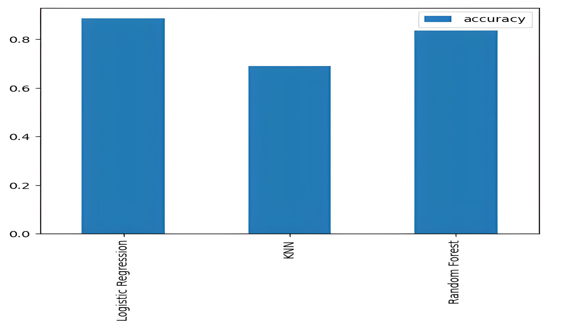
Baseline Results

The models were evaluated using accuracy scores:

• Logistic Regression: 88.5%
• KNN: 68.8%
• Random Forest: 83.6%

models = {"Logistic Regression": LogisticRegression(),
          "KNN": KNeighborsClassifier(),
          "Random Forest": RandomForestClassifier()}
model_scores = fit_and_score(models, X_train, X_test, y_train, y_test)

KNN Hyperparameter Tuning

Optimal n_neighbors value improved KNN accuracy to 75.4%.

knn.set_params(n_neighbors=optimal_value)
knn.fit(X_train, y_train)

Logistic Regression Tuning

• Best hyperparameters: C=0.233 and solver="liblinear".
• Final accuracy: 88.5%.

rs_log_reg.best_params_

---

Sample Code: Hyperparameter tuning with RandomizedSearchCV

log_reg_grid = {"C": np.logspace(-4, 4, 20),
                "solver": ["liblinear"]}
# Hyperparameter grid for RandomForestClassifier
rf_grid = {"n_estimators": np.arange(10, 1000, 50),
           "max_depth": [None, 3, 5, 10],
           "min_samples_split": np.arange(2, 20, 2),
           "min_samples_leaf": np.arange(1, 20, 2)}
# Tune LogisticRegression using RandomizedSearchCV
np.random.seed(42)

# Hyperparameter search for LogisticRegression
rs_log_reg = RandomizedSearchCV(LogisticRegression(),
                                param_distributions=log_reg_grid,
                                cv=5,
                                n_iter=20,
                                verbose=True)

# Random hyperparameter search model for LogisticRegression
rs_log_reg.fit(X_train, y_train)

Sample Code: Hyperparamter Tuning with GridSearchCV

# Different hyperparameters for our LogisticRegression model
log_reg_grid = {"C": np.logspace(-4, 4, 30),
                "solver": ["liblinear"]}

# Setup grid hyperparameter search for LogisticRegression
gs_log_reg = GridSearchCV(LogisticRegression(),
                          param_grid=log_reg_grid,
                          cv=5,
                          verbose=True)

# Fit grid hyperparameter search model
gs_log_reg.fit(X_train, y_train);
gs_log_reg.best_params_
gs_log_reg.score(X_test, y_test)

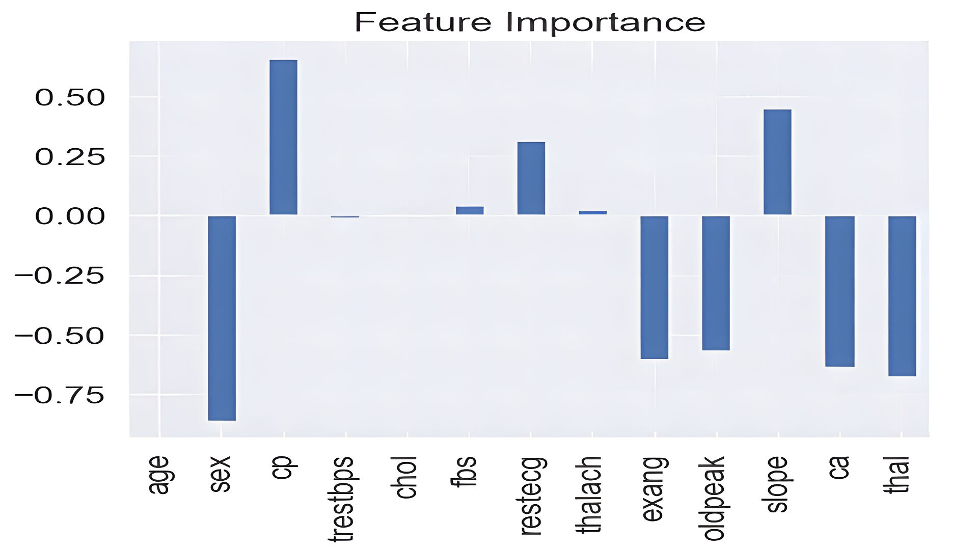
Feature Importance

Logistic Regression coefficients reveal that sex, chest pain type, and thalach (max heart rate) significantly influence predictions.

feature_dict = dict(zip(df.columns, list(clf.coef_[0])))
feature_df.T.plot.bar(title="Feature Importance", legend=False);

---

Conclusion

This project demonstrates the application of machine learning in heart disease prediction. Key outcomes include:

• Logistic Regression emerged as the most accurate model (88.5%).
• Feature importance analysis highlights actionable insights for healthcare.
• Future work can incorporate additional features or ensemble models for higher accuracy.