BTC Predictions Using Deep Learning Models
Overview
This project leverages deep learning models to forecast Bitcoin prices. It includes extensive data preprocessing, feature engineering, and predictive modeling. The goal was to capture Bitcoin's highly volatile and non-linear price dynamics while providing interpretable and accurate predictions.
Key Contributions
-
Data Preprocessing:
- Historical Bitcoin price data was collected and cleaned.
- Features like moving averages, price differences, and lagged returns were engineered.
- Data was scaled to improve model performance.
-
Baseline Models:
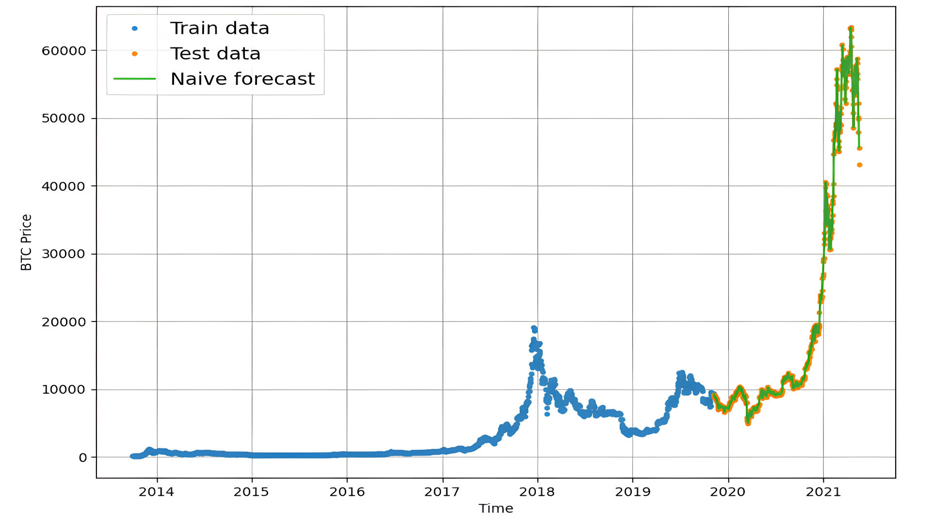
- Naïve forecast is a simple and intuitive time-series forecasting method that assumes the value at the next time step will be equal to the value at the current time step (or a recent average, depending on the context). It serves as a baseline model to compare more sophisticated forecasting methods.
Mapping the forcast to our data:
Evaulating the Naive-Forcast prediction:
import tensorflow as tf

# Implement MASE (assuming no seasonality of data).

def mean_absolute_scaled_error(y_true, y_pred):

  mae = tf.reduce_mean(tf.abs(y_true - y_pred))

  # Finding the MAE of naive forecast (no seasonality)
  mae_naive_no_season = tf.reduce_mean(tf.abs(y_true[1:] - y_true[:-1])) # our seasonality is 1 day (hence the shifting of 1 day)

  return mae / mae_naive_no_season

def evaluate_preds(y_true, y_pred):
  # Make sure float32 (for metric calculations)
  y_true = tf.cast(y_true, dtype=tf.float32)
  y_pred = tf.cast(y_pred, dtype=tf.float32)

  # Calculate various metrics
  mae = tf.keras.metrics.mean_absolute_error(y_true, y_pred)
  mse = tf.keras.metrics.mean_squared_error(y_true, y_pred) # puts and emphasis on outliers (all errors get squared)
  rmse = tf.sqrt(mse)
  mape = tf.keras.metrics.mean_absolute_percentage_error(y_true, y_pred)
  mase = mean_absolute_scaled_error(y_true, y_pred)

  return {"mae": mae.numpy(),
          "mse": mse.numpy(),
          "rmse": rmse.numpy(),
          "mape": mape.numpy(),
          "mase": mase.numpy()}

naive_results = evaluate_preds(y_true=y_test[1:],
                               y_pred=naive_forecast)
naive_results
Outputed the following Evaluation Metrics:
Mean Absolute Error (MAE)
- Definition: The average of the absolute differences between forecasted and actual values.
- Formula:
- Value: 567.9802
- Interpretation: On average, the model’s predictions deviate by 567.98 units from the actual values. For Bitcoin prices, this indicates moderate errors.
Mean Squared Error (MSE)
- Definition: The average of the squared differences between forecasted and actual values.
- Formula:
- Value: 1,147,547.0
- Interpretation: The MSE penalizes larger errors more heavily, indicating the presence of significant deviations in some predictions.
Root Mean Squared Error (RMSE)
- Definition: The square root of the MSE, providing error in the same units as the data.
- Formula:
- Value: 1,071.2362
- Interpretation: On average, the model's predictions are off by 1,071.23 units, indicating notable error compared to the Bitcoin price scale.
Mean Absolute Percentage Error (MAPE)
- Definition: The average percentage error between forecasted and actual values.
- Formula:
- Value: 2.516525
- Interpretation: The model achieves a relatively low error of 2.52%, which suggests good performance in relative terms.
Mean Absolute Scaled Error (MASE)
- Definition: Compares the forecast error to a baseline forecast, such as a naïve forecast.
- Formula:
- Value: 0.99957
- Interpretation: The model performs similarly to a naïve forecast. Its performance improvement over the baseline is minimal.
I then created 3 new models to evaluate against our baseline model.
Model 1:
def make_preds(model, input_data):
  forecast = model.predict(input_data)
  return tf.squeeze(forecast)

model_1_preds = make_preds(model_1, test_windows)
len(model_1_preds), model_1_preds[:10]

# Evaluate preds
model_1_results = evaluate_preds(y_true=tf.squeeze(test_labels), # reduce to right shape
                                 y_pred=model_1_preds)
model_1_results
Model 2:
HORIZON = 1 # predict one step at a time
WINDOW_SIZE = 30 # use 30 timesteps in the past

full_windows, full_labels = make_windows(prices, window_size=WINDOW_SIZE, horizon=HORIZON)
len(full_windows), len(full_labels)

train_windows, test_windows, train_labels, test_labels = make_train_test_splits(windows=full_windows, labels=full_labels)
len(train_windows), len(test_windows), len(train_labels), len(test_labels)

tf.random.set_seed(42)

# Create model (same model as model 1 but data input will be different)
model_2 = tf.keras.Sequential([
  layers.Dense(128, activation="relu"),
  layers.Dense(HORIZON)
], name="model_2_dense")

model_2.compile(loss="mae",
                optimizer=tf.keras.optimizers.Adam())

model_2.fit(train_windows,
            train_labels,
            epochs=100,
            batch_size=128,
            verbose=0,
            validation_data=(test_windows, test_labels),
            callbacks=[create_model_checkpoint(model_name=model_2.name)])

model_2.evaluate(test_windows, test_labels)

# Loading in best performing model
model_2 = tf.keras.models.load_model("model_experiments/model_2_dense/")
model_2.evaluate(test_windows, test_labels)

model_2_preds = make_preds(model_2,
                           input_data=test_windows)

# Evaluate results for model 2 predictions
model_2_results = evaluate_preds(y_true=tf.squeeze(test_labels), # remove 1 dimension of test labels
                                 y_pred=model_2_preds)
model_2_results
Model 3:
HORIZON = 7
WINDOW_SIZE = 30

full_windows, full_labels = make_windows(prices, window_size=WINDOW_SIZE, horizon=HORIZON)
len(full_windows), len(full_labels)

train_windows, test_windows, train_labels, test_labels = make_train_test_splits(windows=full_windows, labels=full_labels, test_split=0.2)
len(train_windows), len(test_windows), len(train_labels), len(test_labels)

tf.random.set_seed(42)

# Create model (same as model_1 except with different data input size)
model_3 = tf.keras.Sequential([
  layers.Dense(128, activation="relu"),
  layers.Dense(HORIZON)
], name="model_3_dense")

model_3.compile(loss="mae",
                optimizer=tf.keras.optimizers.Adam())

model_3.fit(train_windows,
            train_labels,
            batch_size=128,
            epochs=100,
            verbose=0,
            validation_data=(test_windows, test_labels),
            callbacks=[create_model_checkpoint(model_name=model_3.name)])


model_3.evaluate(test_windows, test_labels)

model_3 = tf.keras.models.load_model("model_experiments/model_3_dense/")
model_3.evaluate(test_windows, test_labels)

model_3_preds = make_preds(model_3,
                           input_data=test_windows)
model_3_preds[:5]

model_3_results = evaluate_preds(y_true=tf.squeeze(test_labels),
                                 y_pred=model_3_preds)
model_3_results
1. Model Architecture
All models share a similar architecture:
- Layers:
- A dense layer with 128 units and ReLU activation.
- An output dense layer, with neurons equal to the forecasting horizon.
- Loss Function: Mean Absolute Error (MAE).
The primary difference lies in the input structure and the forecasting horizon.
2. Input and Forecasting Horizon
-
Model 1:
- Input: A window size of 30 past timesteps to predict the next 1 timestep (HORIZON = 1).
- Goal: Short-term prediction, one step at a time.
- Performance:
- mae: 563.3081 (slightly better than the naïve baseline).
-
Model 2:
- Input: Similar to Model 1 but trained and validated on different splits.
- Goal: Short-term prediction.
- Performance:
- mae: 596.4838 (slightly worse than Model 1 and the baseline).
-
Model 3:
- Input: A window size of 30 to predict the next 7 timesteps (HORIZON = 7).
- Goal: Multistep forecasting over a longer horizon.
- Performance:
- mae: 1216.8206, reflecting the difficulty of multistep forecasting.
3. Performance Metrics
-
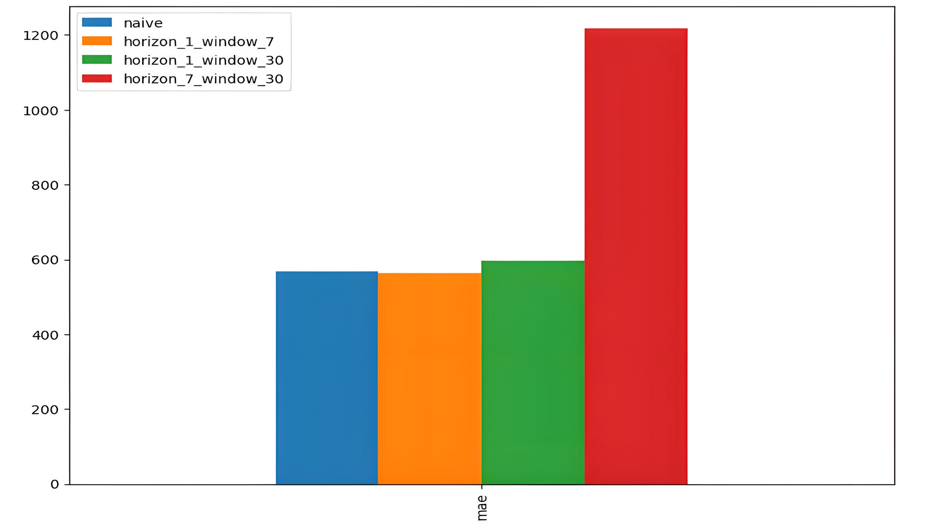
MAE (Mean Absolute Error):
- model_1: 563.3081 (best performance).
- model_2: 596.4838.
- model_3: 1216.8206 (significant error increase for multistep forecasting).
-
MSE and RMSE:
- Both increase significantly for model_3 due to compounding errors over multiple steps.
-
MAPE (Mean Absolute Percentage Error):
- model_1: 2.5269578%.
- model_2: 2.7058904%.
- model_3: 5.464274%, indicating higher relative error.
-
MASE (Mean Absolute Scaled Error):
- model_1: 0.98957634 (better than naïve baseline).
- model_3: 2.1652641 (worse than baseline).
Then plotting the comparison between the two models.
Model 4: Convolutional Neural Network (Conv1D)
Incorporate sequence-to-sequence models or attention mechanisms for multistep forecasting,will improve data prediction. Use external features like trading volume and sentiment data to enhance predictions.Taking account of the pervious models, I created Conv1D, which is great for time-seires forecasting Conv1D is often used to find patterns or trends from sequential data.
Input Data
- Window Size: Uses the past 7 days of data WINDOW_SIZE = 7 to predict the next day's price HORIZON = 1.
- Input Shape Transformation: Data is reshaped from (7,) to (7, 1) using a Lambda layer to make it compatible with the Conv1D layer, which expects a 3D tensor in the format `(batch size, timesteps, features).
Architecture
- Lambda Layer: Expands input dimensions to (7, 1).
- Conv1D Layer:
- Filters: 128 filters extract 128 different patterns from the input sequence.
- Kernel Size: A kernel size of 5 enables the model to analyze local patterns over 5 consecutive timesteps.
- Padding: "Causal" padding ensures predictions are based only on past data, crucial for time-series forecasting.
- Activation Function: ReLU introduces non-linearity to learn complex patterns.
- Dense Layer: A single output neuron predicts the next day's price.
Training
- Loss Function: Mean Absolute Error (MAE).
- Optimizer: Adam optimizer for efficient gradient updates.
- Batch Size: 128, balancing training efficiency and convergence.
- Epochs: Trained for 100 epochs with early stopping and validation monitoring.
Evaluation Results
- MAE: 568.449, slightly better than the naïve baseline (567.9802), indicating comparable accuracy.
- RMSE: 1080.381, reflecting moderate error when considering the scale of Bitcoin prices.
- MAPE: 2.53%, showcasing low relative error and good performance.
- MASE: 0.9986, suggesting performance nearly identical to the naïve baseline.
HORIZON = 1 # predict next day
WINDOW_SIZE = 7 # use previous week worth of data

# Create windowed dataset
full_windows, full_labels = make_windows(prices, window_size=WINDOW_SIZE, horizon=HORIZON)
len(full_windows), len(full_labels)

train_windows, test_windows, train_labels, test_labels = make_train_test_splits(full_windows, full_labels)
len(train_windows), len(test_windows), len(train_labels), len(test_labels)

train_windows[0].shape

# In order to ensure functionality, we must modify the structure of our data before feeding it into the Conv1D layer.
x = tf.constant(train_windows[0])
expand_dims_layer = layers.Lambda(lambda x: tf.expand_dims(x, axis=1))
print(f"Original shape: {x.shape}") # (WINDOW_SIZE)
print(f"Expanded shape: {expand_dims_layer(x).shape}") # (WINDOW_SIZE, input_dim)
print(f"Original values with expanded shape:\n {expand_dims_layer(x)}")

tf.random.set_seed(42)

# Create model
model_4 = tf.keras.Sequential([
  layers.Lambda(lambda x: tf.expand_dims(x, axis=1)),
  layers.Conv1D(filters=128, kernel_size=5, padding="causal", activation="relu"),
  layers.Dense(HORIZON)
], name="model_4_conv1D")

# Compile model
model_4.compile(loss="mae",
                optimizer=tf.keras.optimizers.Adam())

# Fit model
model_4.fit(train_windows,
            train_labels,
            batch_size=128,
            epochs=100,
            verbose=0,
            validation_data=(test_windows, test_labels),
            callbacks=[create_model_checkpoint(model_name=model_4.name)])

model_4 = tf.keras.models.load_model("model_experiments/model_4_conv1D")
model_4.evaluate(test_windows, test_labels)

# Making predictions
model_4_preds = make_preds(model_4, test_windows)
model_4_preds[:10]

model_4_results = evaluate_preds(y_true=tf.squeeze(test_labels),
                                 y_pred=model_4_preds)
model_4_results
Recurrent Neural Networks (RNNs)
Another Model we can use for the sequential data is a Recurrent Neural Net or in Our case an LSTM model. Recurrent Neural Networks introduce a mechanism where the output from one step is fed back as input to the next, allowing them to retain information from previous inputs. This design makes RNNs well-suited for tasks where context from earlier steps is essential, such as predicting the next word in a sentence.
Definition adapted from
Introduction to Recurrent Neural Networks
Model 5: Recurrent Neural Network (LSTM)
Input Data
- Window Size: Past 7 days of prices WINDOW_SIZE = 7 to predict the next day HORIZON = 1.
- Input shape expanded from (7,) to (7, 1) for compatibility with the LSTM layer.
Architecture
- LSTM Layer: 128 units with ReLU activation to capture temporal dependencies.
- Dense Layer: Outputs the next day’s predicted price.
Evaluation
- MAE: 582.4414
- MAPE: 2.63% (low relative error).
- Performance slightly better than the naïve baseline.
tf.random.set_seed(42)
inputs = layers.Input(shape=(WINDOW_SIZE))
x = layers.Lambda(lambda x: tf.expand_dims(x, axis=1))(inputs)
x = layers.LSTM(128, activation="relu")(x)
output = layers.Dense(HORIZON)(x)
model_5 = tf.keras.Model(inputs=inputs, outputs=output, name="model_5_lstm")

# Compile model
model_5.compile(loss="mae",
                optimizer=tf.keras.optimizers.Adam())

model_5.fit(train_windows,
            train_labels,
            epochs=100,
            verbose=0,
            batch_size=128,
            validation_data=(test_windows, test_labels),
            callbacks=[create_model_checkpoint(model_name=model_5.name)])

model_5 = tf.keras.models.load_model("model_experiments/model_5_lstm/")
model_5.evaluate(test_windows, test_labels)

# Make predictions with our LSTM model
model_5_preds = make_preds(model_5, test_windows)
model_5_preds[:10]

# Evaluate model 5 preds
model_5_results = evaluate_preds(y_true=tf.squeeze(test_labels),
                                 y_pred=model_5_preds)
model_5_results
Model 6: Multivariate Dense Model
Input Data
- Combines historical prices and block rewards as features for multivariate prediction.
- Includes lagged price values (WINDOW_SIZE = 7).
Architecture
- Two dense layers process multivariate input, with one neuron outputting the predicted price.
Evaluation
- MAE: 562.7571 (best among models).
- MAPE: 2.51% (lowest relative error).
X = bitcoin_prices_windowed.dropna().drop("Price", axis=1).astype(np.float32)
y = bitcoin_prices_windowed.dropna()["Price"].astype(np.float32)
X.head()
y.head()

# training and test sets
split_size = int(len(X) * 0.8)
X_train, y_train = X[:split_size], y[:split_size]
X_test, y_test = X[split_size:], y[split_size:]
len(X_train), len(y_train), len(X_test), len(y_test)

tf.random.set_seed(42)
model_6 = tf.keras.Sequential([
  layers.Dense(128, activation="relu"),
  layers.Dense(HORIZON)
], name="model_6_dense_multivariate")

# Compile
model_6.compile(loss="mae",
                optimizer=tf.keras.optimizers.Adam())

# Fit
model_6.fit(X_train, y_train,
            epochs=100,
            batch_size=128,
            verbose=0, # only print 1 line per epoch
            validation_data=(X_test, y_test),
            callbacks=[create_model_checkpoint(model_name=model_6.name)])

model_6 = tf.keras.models.load_model("model_experiments/model_6_dense_multivariate")
model_6.evaluate(X_test, y_test)

# Making predictions on multivariate data
model_6_preds = tf.squeeze(model_6.predict(X_test))
model_6_preds[:10]

# Evaluate preds
model_6_results = evaluate_preds(y_true=y_test,
                                 y_pred=model_6_preds)
model_6_results
Model 7: N-BEATS
The Neural Basis Expansion Analysis (NBEATS) is an MLP-based deep neural architecture with backward and forward residual links. The network has two variants: (1) in its interpretable configuration, NBEATS sequentially projects the signal into polynomials and harmonic basis to learn trend and seasonality components; (2) in its generic configuration, it substitutes the polynomial and harmonic basis for identity basis and larger network’s depth. The Neural Basis Expansion Analysis with Exogenous (NBEATSx), incorporates projections to exogenous temporal variables available at the time of the prediction.
Definition adapted from
NBEATS
1. Custom N-BEATS Block
The N-BEATS block decomposes time-series data into backcast (residuals) and forecast components, forming the building block of the architecture.
class NBeatsBlock(tf.keras.layers.Layer):
    def __init__(self, input_size, theta_size, horizon, n_neurons, n_layers, **kwargs):
        super().__init__(**kwargs)
        self.hidden = [tf.keras.layers.Dense(n_neurons, activation="relu") for _ in range(n_layers)]
        self.theta_layer = tf.keras.layers.Dense(theta_size, activation="linear", name="theta")

    def call(self, inputs):
        x = inputs
        for layer in self.hidden:
            x = layer(x)
        theta = self.theta_layer(x)
        backcast, forecast = theta[:, :self.input_size], theta[:, -self.horizon:]
        return backcast, forecast

# Test the block with dummy inputs
dummy_inputs = tf.expand_dims(tf.range(7) + 1, axis=0)  # Example input for WINDOW_SIZE = 7
dummy_block = NBeatsBlock(input_size=7, theta_size=8, horizon=1, n_neurons=128, n_layers=4)
backcast, forecast = dummy_block(dummy_inputs)
print(f"Backcast: {tf.squeeze(backcast.numpy())}, Forecast: {tf.squeeze(forecast.numpy())}")
2. Preparing the Dataset
The dataset is structured into rolling windows for forecasting, aligning with the N-BEATS architecture's input format.
# Add windowed columns for Bitcoin prices
WINDOW_SIZE = 7
bitcoin_prices_nbeats = bitcoin_prices.copy()
for i in range(WINDOW_SIZE):
    bitcoin_prices_nbeats[f"Price+{i+1}"] = bitcoin_prices_nbeats["Price"].shift(periods=i+1)
bitcoin_prices_nbeats = bitcoin_prices_nbeats.dropna()

# Split the dataset into training and testing sets
X = bitcoin_prices_nbeats.drop("Price", axis=1)
y = bitcoin_prices_nbeats["Price"]
split_size = int(len(X) * 0.8)
X_train, X_test = X[:split_size], X[split_size:]
y_train, y_test = y[:split_size], y[split_size:]

# Convert to TensorFlow datasets
train_features_dataset = tf.data.Dataset.from_tensor_slices(X_train)
train_labels_dataset = tf.data.Dataset.from_tensor_slices(y_train)
test_features_dataset = tf.data.Dataset.from_tensor_slices(X_test)
test_labels_dataset = tf.data.Dataset.from_tensor_slices(y_test)

train_dataset = tf.data.Dataset.zip((train_features_dataset, train_labels_dataset)).batch(1024).prefetch(tf.data.AUTOTUNE)
test_dataset = tf.data.Dataset.zip((test_features_dataset, test_labels_dataset)).batch(1024).prefetch(tf.data.AUTOTUNE)
3. Building the N-BEATS Model
The model consists of multiple stacked N-BEATS blocks with residual stacking to improve predictions.
# Define input parameters
N_EPOCHS = 5000
N_NEURONS = 512
N_LAYERS = 4
N_STACKS = 30
INPUT_SIZE = WINDOW_SIZE
THETA_SIZE = WINDOW_SIZE + 1

# Initialize N-BEATS block
stack_input = layers.Input(shape=(INPUT_SIZE), name="stack_input")
nbeats_block = NBeatsBlock(input_size=INPUT_SIZE, theta_size=THETA_SIZE, horizon=1, n_neurons=N_NEURONS, n_layers=N_LAYERS)
backcast, forecast = nbeats_block(stack_input)

# Residual stacking
residuals = layers.subtract([stack_input, backcast], name="subtract_00")
for i in range(N_STACKS - 1):
    block = NBeatsBlock(input_size=INPUT_SIZE, theta_size=THETA_SIZE, horizon=1, n_neurons=N_NEURONS, n_layers=N_LAYERS)
    backcast, block_forecast = block(residuals)
    residuals = layers.subtract([residuals, backcast], name=f"subtract_{i}")
    forecast = layers.add([forecast, block_forecast], name=f"add_{i}")

# Final model
model_7 = tf.keras.Model(inputs=stack_input, outputs=forecast, name="model_7_N-BEATS")
model_7.compile(loss="mae", optimizer=tf.keras.optimizers.Adam(0.001), metrics=["mae", "mse"])
4. Training and Evaluation
The model is trained with callbacks to handle early stopping and learning rate reduction.
# Train the model
model_7.fit(
    train_dataset,
    validation_data=test_dataset,
    epochs=N_EPOCHS,
    callbacks=[
        tf.keras.callbacks.EarlyStopping(monitor="val_loss", patience=200, restore_best_weights=True),
        tf.keras.callbacks.ReduceLROnPlateau(monitor="val_loss", patience=100, verbose=1),
    ]
)

# Evaluate the model
results = model_7.evaluate(test_dataset)
print(f"MAE: {results[1]}, MSE: {results[2]}")

# Make predictions
model_7_preds = make_preds(model_7, test_dataset)
print(f"Predictions: {model_7_preds[:10]}")
5. Results
The N-BEATS model achieved the following metrics:
- MAE: 574.2568
- MSE: 1,132,843.9
- RMSE: 1,064.3513
- MAPE: 2.63%
Constructing and Fitting Ensemble Models
This process involves building and training multiple models with varying loss functions, aggregating their predictions to create a robust ensemble model for time-series forecasting.
1. Ensemble Model Construction
The ensemble consists of multiple individual models trained with different configurations to optimize performance.
Key Components:
-
Input Parameters:
- horizon: Defines the forecasting horizon (number of steps to predict).
- num_iter: Number of iterations per loss function to train models.
- num_epochs: Number of training epochs per model.
- loss_fns: List of loss functions to optimize (mae, mse, mape).
-
Model Architecture:
- Each model is a simple feedforward neural network with:
- Two hidden layers (128 neurons each, ReLU activation).
- One output layer matching the horizon.
- Each model is a simple feedforward neural network with:
-
Compilation:
- Models are compiled with the specified loss function and the Adam optimizer.
- Metrics include mae and mse.
-
Training:
- Each model is trained on the training dataset and validated on the test dataset.
- Early stopping and learning rate reduction callbacks are used to prevent overfitting and optimize training.
Code Sample: Model Construction
def get_ensemble_models(horizon=HORIZON,
                        train_data=train_dataset,
                        test_data=test_dataset,
                        num_iter=10,
                        num_epochs=100,
                        loss_fns=["mae", "mse", "mape"]):
    # List to store trained ensemble models
    ensemble_models = []

    for i in range(num_iter):
        for loss_function in loss_fns:
            print(f"Optimizing model with loss: {loss_function}, model number: {i}")

            # Define the model architecture
            model = tf.keras.Sequential([
                layers.Dense(128, kernel_initializer="he_normal", activation="relu"),
                layers.Dense(128, kernel_initializer="he_normal", activation="relu"),
                layers.Dense(horizon)
            ])

            # Compile the model
            model.compile(
                loss=loss_function,
                optimizer=tf.keras.optimizers.Adam(),
                metrics=["mae", "mse"]
            )

            # Train the model
            model.fit(
                train_data,
                epochs=num_epochs,
                verbose=0,
                validation_data=test_data,
                callbacks=[
                    tf.keras.callbacks.EarlyStopping(monitor="val_loss", patience=200, restore_best_weights=True),
                    tf.keras.callbacks.ReduceLROnPlateau(monitor="val_loss", patience=100, verbose=1)
                ]
            )

            # Add the trained model to the ensemble list
            ensemble_models.append(model)

    return ensemble_models

# Train ensemble models
ensemble_models = get_ensemble_models(num_iter=5, num_epochs=1000)
2. Making Predictions with the Ensemble
The ensemble's predictions are computed by aggregating the outputs of all individual models, typically using the median to reduce the influence of outliers.
Steps:
- Generate Predictions:
- Each model in the ensemble predicts the test dataset.
- Aggregate Predictions:
- Use the median of predictions across all models as the final ensemble output.
Code Sample: Prediction Aggregation
def make_ensemble_preds(ensemble_models, data):
    ensemble_preds = []
    for model in ensemble_models:
        preds = model.predict(data)
        ensemble_preds.append(preds)
    return tf.constant(tf.squeeze(ensemble_preds))

# Generate ensemble predictions
ensemble_preds = make_ensemble_preds(ensemble_models=ensemble_models, data=test_dataset)
3. Evaluating the Ensemble Model
The aggregated predictions are evaluated against the true labels using metrics like mae, mse, rmse, and mape.
Code Sample: Evaluation
# Evaluate the ensemble model
ensemble_results = evaluate_preds(
    y_true=y_test,
    y_pred=np.median(ensemble_preds, axis=0)
)
ensemble_results
Advantages of Ensemble Models
- Robustness:
- Reduces variance and overfitting compared to individual models.
- Performance:
- Combines strengths of multiple loss functions for better generalization.
- Flexibility:
- Can adapt to various forecasting horizons and data patterns.
Bootstrapping the Models for Prediction Intervals
Bootstrapping is a statistical method used to estimate the uncertainty of model predictions. In this context, the predictions from the ensemble models are bootstrapped to calculate prediction intervals.
1. Calculating Prediction Intervals
The prediction intervals are derived using the standard deviation of the predictions from the ensemble models. A 95% confidence interval is computed using the formula:
Where:
- is the mean of predictions.
- is the standard deviation of predictions.
Code Implementation:
def get_upper_lower(preds):
    # Calculate standard deviation across ensemble predictions
    std = tf.math.reduce_std(preds, axis=0)

    # Compute 95% prediction interval
    interval = 1.96 * std

    # Calculate mean predictions
    preds_mean = tf.reduce_mean(preds, axis=0)

    # Compute lower and upper bounds
    lower, upper = preds_mean - interval, preds_mean + interval
    return lower, upper

# Compute prediction intervals for ensemble predictions
lower, upper = get_upper_lower(preds=ensemble_preds)
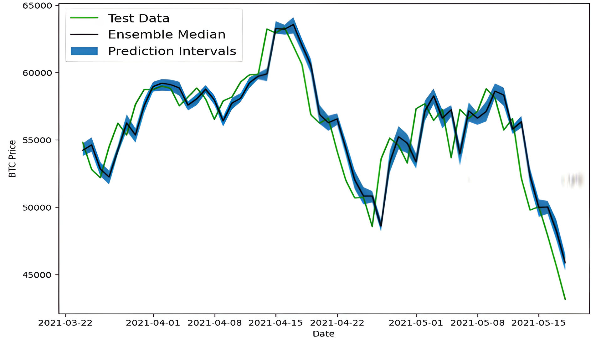
2. Visualization
The results are visualized by plotting:
- Test Data: Ground truth values for Bitcoin prices.
- Ensemble Median: Median predictions from the ensemble models.
- Prediction Intervals: Shaded area between the lower and upper bounds of the 95% confidence interval.
Code Implementation:
import matplotlib.pyplot as plt

# Plot ensemble median with prediction intervals
ensemble_median = np.median(ensemble_preds, axis=0)
offset = 500  # Start plotting from this offset to reduce clutter

plt.figure(figsize=(10, 7))
plt.plot(X_test.index[offset:], y_test[offset:], "g", label="Test Data")
plt.plot(X_test.index[offset:], ensemble_median[offset:], "k-", label="Ensemble Median")
plt.fill_between(X_test.index[offset:],
                 lower[offset:],
                 upper[offset:],
                 color="gray", alpha=0.3, label="Prediction Intervals")
plt.xlabel("Date")
plt.ylabel("BTC Price")
plt.legend(loc="upper left", fontsize=14)
plt.title("Ensemble Predictions with 95% Prediction Intervals")
plt.show()
3. Insights from the Visualization
-
Ensemble Median:
- Represents the central tendency of predictions from the ensemble models.
- Smooths out fluctuations in individual predictions.
-
Prediction Intervals:
- Provide a range within which the true Bitcoin price is expected to fall with 95% confidence.
- Wider intervals indicate higher uncertainty in predictions.
-
Comparison to Test Data:
- Allows for evaluating how closely the predictions align with actual prices.
Advantages of Bootstrapping
- Quantifies Uncertainty: Helps assess the reliability of predictions.
- Improves Robustness: Aggregates insights from multiple models.
- Visual Interpretability: Provides intuitive confidence bands for predictions.
Training the Model for Next-Day Price Prediction
A 7-day windowed dataset is used to train a feedforward neural network for forecasting Bitcoin prices.
1. Data Preparation
Create a windowed dataset with 7-day inputs and the next day's price as the target.
X_all = bitcoin_prices_windowed.drop(["Price", "block_reward"], axis=1).dropna().to_numpy()
y_all = bitcoin_prices_windowed.dropna()["Price"].to_numpy()
dataset_all = tf.data.Dataset.from_tensor_slices((X_all, y_all)).batch(1024).prefetch(tf.data.AUTOTUNE)
2. Model Training
Train a simple feedforward neural network with two hidden layers.
model_9 = tf.keras.Sequential([
  layers.Dense(128, activation="relu"),
  layers.Dense(128, activation="relu"),
  layers.Dense(1)  # Predict 1 day ahead
])

model_9.compile(loss="mae", optimizer="adam")
model_9.fit(dataset_all, epochs=100, verbose=0)
3. Forecasting
Predict future prices iteratively using the most recent 7-day window.
def make_future_forecast(values, model, into_future, window_size=7):
    future_forecast = []
    last_window = values[-window_size:]
    for _ in range(into_future):
        future_pred = model.predict(tf.expand_dims(last_window, axis=0))
        future_forecast.append(tf.squeeze(future_pred).numpy())
        last_window = np.append(last_window, future_pred)[-window_size:]
    return future_forecast

future_forecast = make_future_forecast(y_all, model_9, into_future=14)
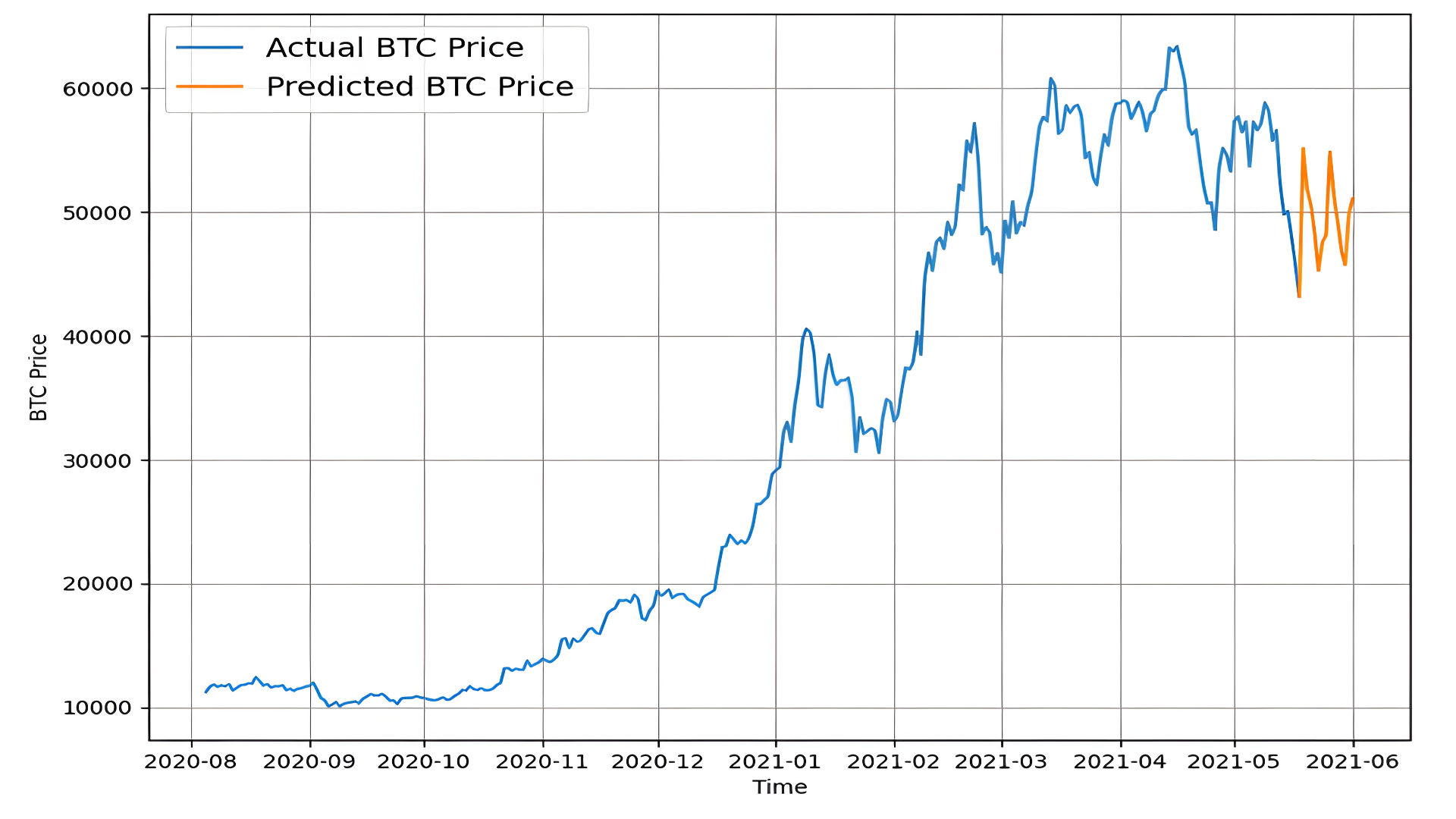
4. Visualization
Plot actual and predicted prices.
plot_time_series(bitcoin_prices.index, btc_price, label="Actual BTC Price")
plot_time_series(get_future_dates(bitcoin_prices.index[-1], 14), future_forecast, label="Predicted BTC Price")
plt.show()
Summary
- Predicts next-day prices using a 7-day window.
- Extends predictions iteratively for multiple days.
- Ideal for short-term Bitcoin trend forecasting.
Conclusion
This project showcases the application of deep learning models for Bitcoin price prediction. It highlights how sequential data and neural networks can effectively forecast cryptocurrency prices. Below are the key takeaways and potential avenues for future exploration:
Key Achievements
-
Baseline Comparisons:
- Developed baseline models, including a naïve forecast, for robust comparison.
- Showed how advanced models improve upon simple benchmarks.
-
Advanced Model Architectures:
- Explored diverse architectures: dense networks, Conv1D, LSTM, and N-BEATS.
- Evaluated model performance using metrics such as MAE, MSE, RMSE, and MAPE.
-
Ensemble Learning:
- Enhanced prediction accuracy and robustness through ensemble modeling.
- Used bootstrapping to provide 95% prediction intervals, quantifying model uncertainty.
-
Short- and Long-Term Forecasting:
- Models were capable of both single-step (next-day) and multistep forecasting, adapting to various horizons.
-
Visualization and Interpretability:
- Provided clear visual comparisons between actual and predicted prices.
- Demonstrated the effectiveness of prediction intervals in assessing uncertainty.
Challenges and Insights
- Data Volatility: Bitcoin's inherent volatility adds complexity to modeling, requiring robust architectures like LSTM and N-BEATS.
- Multistep Forecasting: Longer horizons introduce cumulative errors, emphasizing the need for specialized techniques like sequence-to-sequence models.
- Baseline Performance: Models must consistently outperform naïve forecasts to justify complexity.
Future Directions
-
Incorporate External Data:
- Add features like trading volume, social sentiment, or macroeconomic indicators to improve predictive power.
-
Test Advanced Architectures:
- Experiment with attention mechanisms or transformer models for time-series forecasting.
-
Real-Time Implementation:
- Deploy models in real-time trading environments to assess performance under dynamic market conditions.
-
Explore Financial Metrics:
- Evaluate models based on financial performance metrics like Sharpe Ratio or drawdown in a simulated trading strategy.
Final Thoughts
By employing innovative deep learning techniques, this project not only predicts Bitcoin prices but also offers a methodological framework for handling other financial time-series data. The findings emphasize the balance between complexity and interpretability, providing a strong foundation for further research in cryptocurrency forecasting and quantitative finance.